Building Ridgeline Plots in R with the "ggridges" Package

In this blog post we’ll look at creating Ridgeline Plots in R. A Rigdeline Plot (sometimes referred to as a Joy Plot) is typically used to visualize a single quantitative variable across several categories. In our first example, we will look at how the distribution of daily maximum temperature in Lincoln, Nebraska (a quantitative variable) changes by month (categorical). The second example uses college football data from the “cfbfastR” package cfbfastR R Package. Let’s get started!

R Packages

As we usually do in R, start by installing and loading the necessary packages using R’s “install.packages” and “library” functions. In my code below, I have commented out the “install.packages” functions as I have already installed these libraries and do not need to install them again.

I use Tidyverse functions in virtually all of my R projects and we need access to the “ggplot2” package (part of the Tidyverse) for this work. The Ridgeline plots are created via the “ggridges” package ggridges R Package. As noted above, the “cfbfastR” package will be used to obtain college football data for one of our examples.

#install.packages("tidyverse")
#install.packages("ggridges")
#install.packages("cfbfastR")
library(tidyverse)
library(ggridges)
library(cfbfastR)

Loading the Data

For our first few Ridgeline Plot examples let’s use the “lincoln_weather” dataset that is part of the “ggridges” package. This package contains weather data from the year 2016 from Lincoln, Nebraska. We create a data frame called “lincoln” with the line of code of below.

lincoln = ggridges::lincoln_weather

Ridgeline Plots with the “ggridges” package are created using standard “ggplot2” syntax with the Ridgeline plots provided as a “geom”. Let’s start by building a Ridgeline Plot of temperature by month with histograms. The code here is pretty straightforward. The key is the use of “geom_density_ridges”. Setting “stat” to “binline” allows for histograms rather than smoothed density plots (we’ll see those in a moment). With the exception of the added x and y axis labels, the code here is default. The quantitiative variable “Max Temperature [F]” is placed on the x axis with “Month” on the y axis. Note the use of the backtick symbol (`) around the name of the “Max Temperature [F]” variable. This is necessary because of the spaces present in the variable name.

ggplot(lincoln, aes(x = `Max Temperature [F]`, y = Month)) +
    geom_density_ridges(stat = "binline") +
    xlab("Maximum Temperature [F]") +
    ylab("Month")

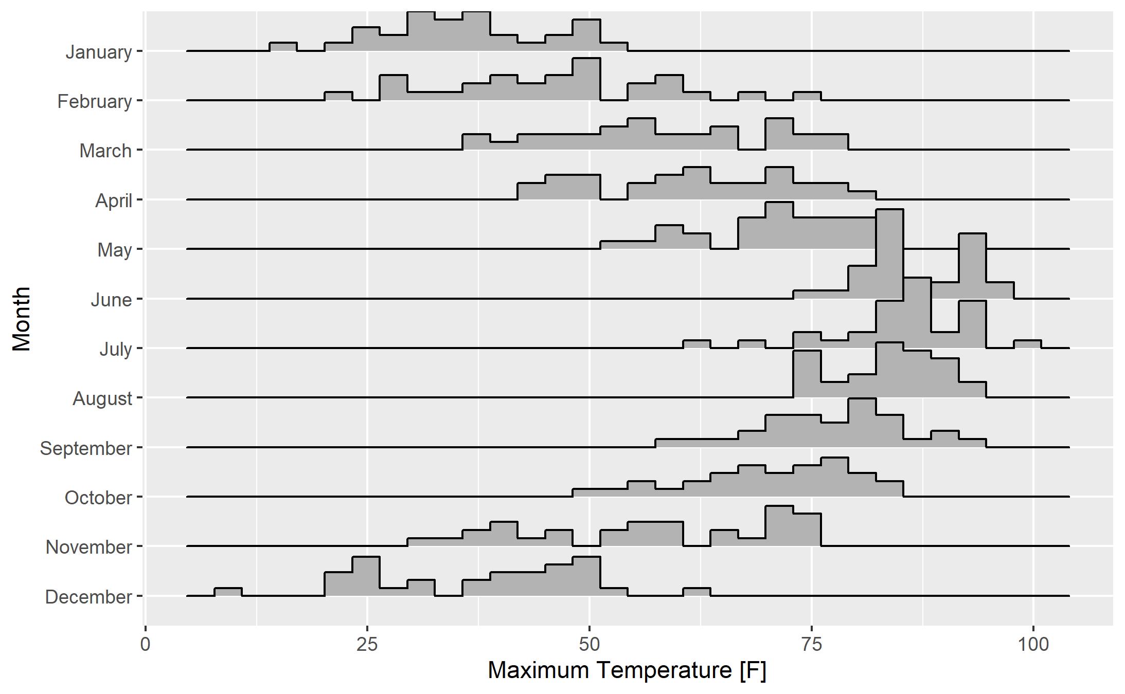
My first reaction to this plot is a resounding “meh”. Let’s make a few changes to see if we can improve the plot:

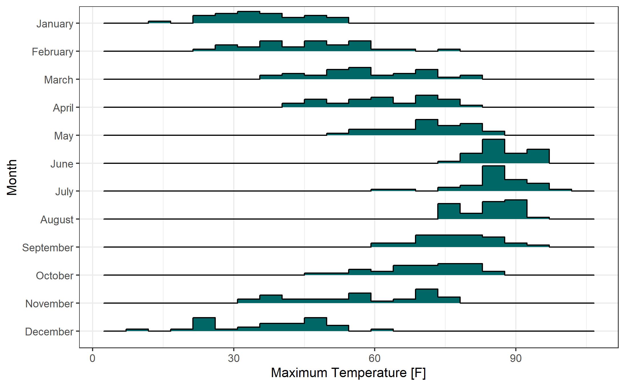
• To reduce the overlap of the histograms (see the June histogram overlapping May, for example) we can change the “scale” parameter in “geom_density_ridges”. A “scale” of 1 sets the height of each category to the height of the tallest histogram bar. Higher values for “scale” allow more overlap. If you don’t mind a bit of overlap, feel free to adjust “scale” to your liking. As you might expect, adjusting “scale” the other direction (less than 1) increases the gap between the tallest histogram bar and the histogram for the category above it.
• The default number of bins for each histogram is 30. That seems like a bit too many for this example, so I changed the number of bins to 20 via the “bins” parameter inside the “geom_density_ridges”.
• Personally, I prefer either the “theme_bw” or “theme_minimal” themes. Here I’ll use theme_bw.
• If you want to change the color that is used to fill the histograms, you can add a “fill” to the “geom_density_ridges”. For precise control of the color, I recommend using color hex codes. Here I use the hex code for UNCW’s teal color.

ggplot(lincoln, aes(x = `Max Temperature [F]`, y = Month)) +
    geom_density_ridges(stat = "binline", bins = 20,scale = 0.9, fill = "#006666") +
    xlab("Maximum Temperature [F]") +
    ylab("Month") +
    theme_bw()

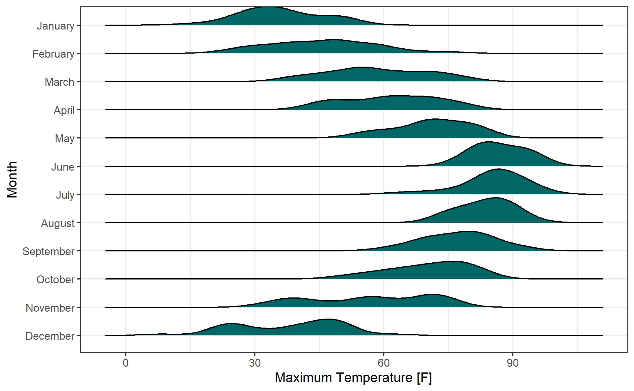
While the histogram-based Ridgeline Plots are nice, I prefer the look of the smoothed density curve version. Here’s the same plot from above with smoothed density curves rather than histograms. Removing the “binline” and “bins” parameters from “geom_density_ridges” yields this plot.

ggplot(lincoln, aes(x = `Max Temperature [F]`, y = Month)) +
    geom_density_ridges(scale = 0.9, fill = "#006666") +
    xlab("Maximum Temperature [F]") +
    ylab("Month") +
    theme_bw()

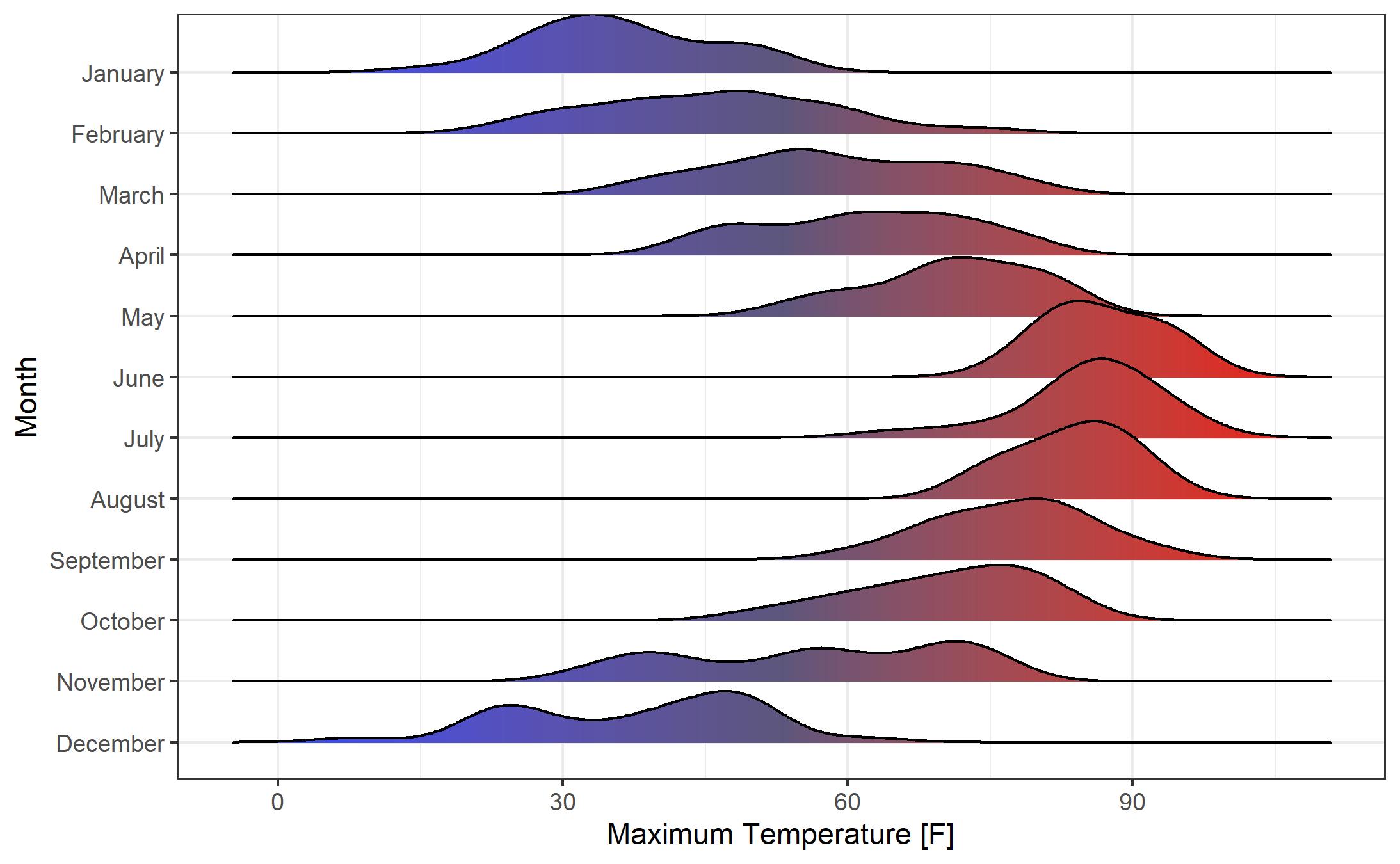
Let’s adjust the scale of the plot. While I’m not normally a fan of “faux 3-D” effects (i.e., the overlap of the smoothed density curves), I think it works pretty well here. We’ll also add a color fill by temperature. Note the syntax for setting up the fill “fill = ..x..” and the change of the geom to “geom_density_ridges_gradient”. We can define the colors of the gradient fill using “scale_fill_gradientn”. The color gradient duplicates information that is shown on the x axis, but adds a pleasant aesthetic to the chart.

ggplot(lincoln, aes(x = `Max Temperature [F]`, y = Month, fill = ..x..)) +
    geom_density_ridges_gradient(scale = 1.3) +
    xlab("Maximum Temperature [F]") +
    ylab("Month") +
    scale_fill_gradientn(colors = c("#194bff", "#5d567c", "#f00a0a")) + 
    theme_bw() + 
    theme(legend.position = "none") 

Using College Football Play-by-Play Data

Now let’s turn our attention to a different dataset. We’ll be using college football play-by-play data from the “cfbfastR” R package. Note that, in order to use this package, you need access to the “CollegeFootballData API”. This access is free. Instructions for obtaining an API key can be found here: cfbfastR Homepage.

We begin by creating an empty data frame that will hold the play-by-play data. We specify which season(s) of data we want to obtain (here we’ll obtain data from the 2020 season). In the next line of code we use the “load_cfb_pbp” function from the “cfbfastR” R package to obtain the play-by-play data and store it in a data frame called “pbp”.

pbp = data.frame()
seasons = 2020
pbp = cfbfastR::load_cfb_pbp(seasons)

We’ll focus our attention on my alma mater, 2020’s National Champion, the Alabama Crimson Tide. We use a “filter” to collect plays for which Alabama was the team in possession or on defense.

bama = pbp %>% filter(pos_team == "Alabama" | def_pos_team == "Alabama")

There is an issue with the play-by-play dataset in that the “week” variable for the two games that Alabama played in the College Football Playoff are incorrectly listed as Weeks 1 and 2. Let’s correct this with a “mutate” function. We then arrange the play-by-play data by week, in descending order.

bama = bama %>% mutate(week = ifelse(def_pos_team == "Notre Dame", 17, week))
bama = bama %>% mutate(week = ifelse(def_pos_team == "Ohio State", 18, week))

bama = bama %>% mutate(def_pos_team = as_factor(def_pos_team)) %>%
    mutate(def_pos_team = fct_reorder(def_pos_team, -week))

Next let’s filter to only look at passing and rushing plays (this will exclude special teams plays, timeouts, etc.) and only at plays where Alabama is in possession. Recall that R’s “or” symbol is “|”.

bama = bama %>% filter(pass == 1 | rush == 1) %>% filter(pos_team == "Alabama")

This leaves us with 1816 plays from 2020 season from games involving Alabama. What should we plot? Let’s look at the distribution of Alabama’s “Expected Points Added” for each play for each game in the season. Expected Points Added (EPA) measures the change in Expected Points from before a play to after the play has occurred. There is a nice explanation of EPA here EPA Explanation.

ggplot(bama, aes(y=def_pos_team, x= EPA)) +
    geom_density_ridges_gradient(aes(scale = 1.3))  +
    xlab("Expected Points Added") +
    ylab("Opponent") + theme_minimal() + 
    theme(legend.position = "none")

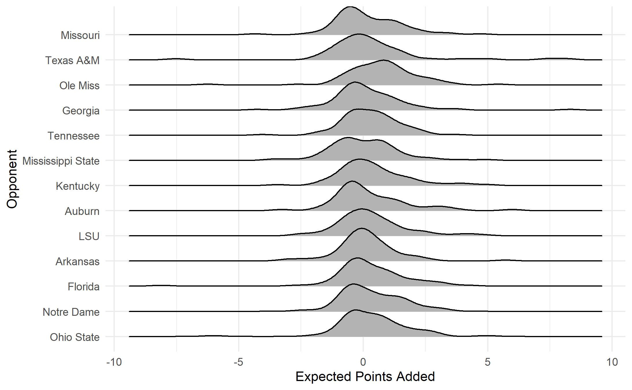
What does this plot show us? Most plays have an EPA value near zero with most values falling between about 2.5 and -2.5. EPA distributions are somewhat similar from game to game. The most notable exception is the game against Ole Miss. This game, won 63-48 by Alabama, featured record-breaking offensive output. Let’s take a closer look at EPA by play type (run versus pass).

We can easily add a second density curve for each category using “fill” inside the “geom_density_ridges” function. Here we fill by the “pass” variable. Note that the pass variable is a numeric variable with a value of 1 if the play is a pass play and a value of 0 if the play is a running play. In the “fill” we make sure that R treats this variable as a factor (a categorical variable).

ggplot(bama, aes(y=def_pos_team, x= EPA)) +
    geom_density_ridges(aes(scale = 1.3, fill = factor(pass)))  +
    xlab("Expected Points Added") +
    ylab("Opponent") + theme_minimal() 

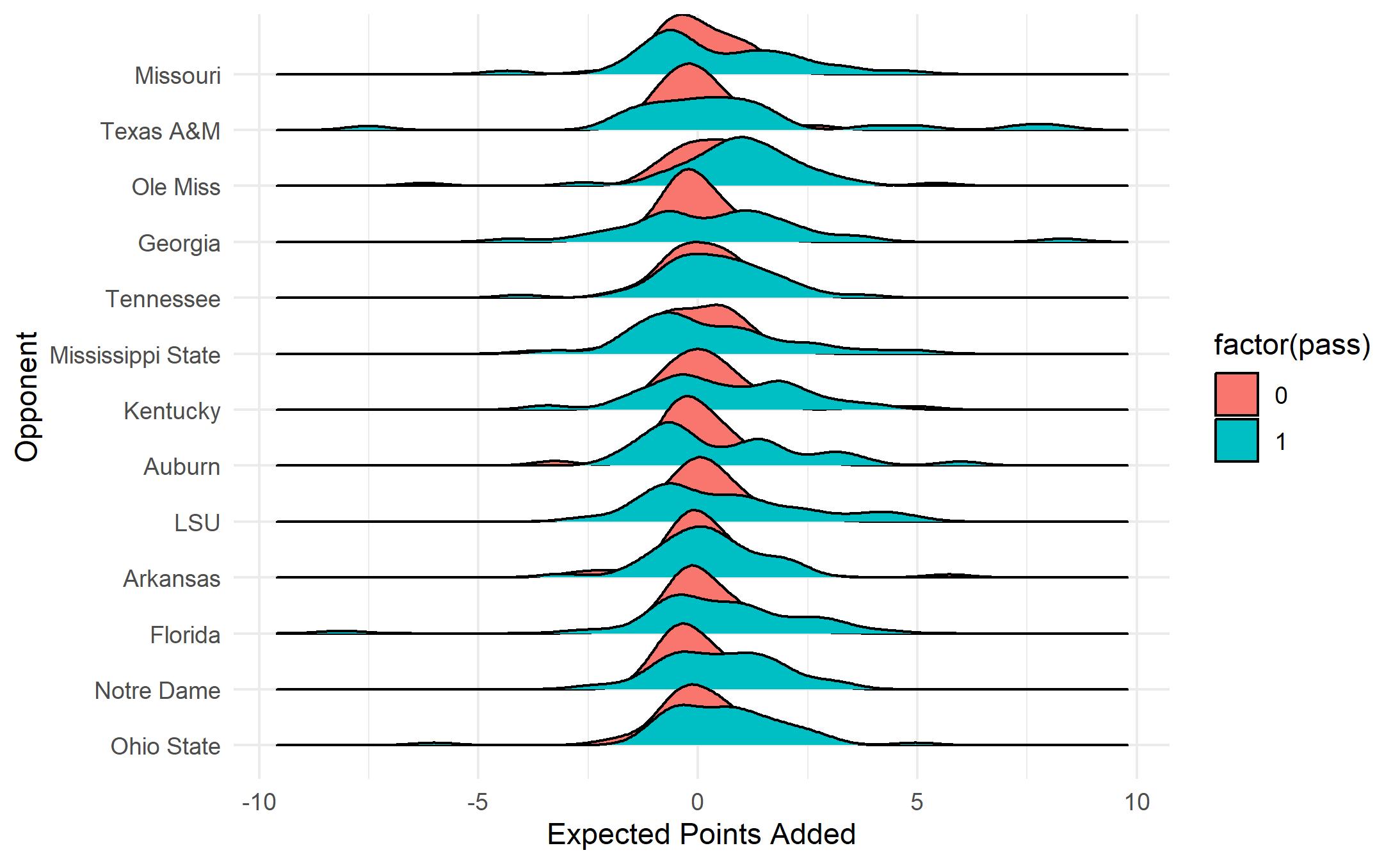
This plot is successful in that it tells the basic story that passing plays tend to have more EPA variance than rushing plays, however, the plot itself leaves a lot to be desired. How can we clean it up?

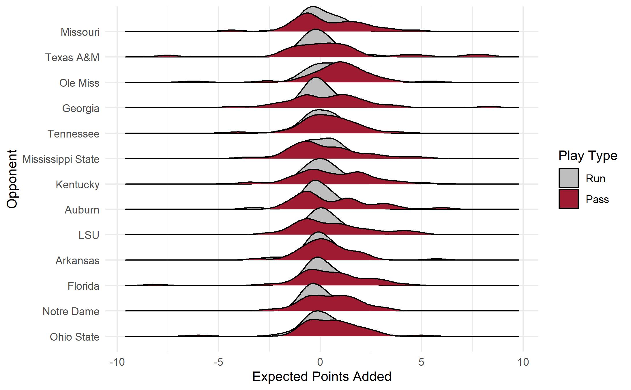
• Adjust the scale slightly to reduce overlap from game to game.
• Adjust the density curve fill colors (mapped to Alabama’s crimson color and a light gray)
• Adjust the legend labels

ggplot(bama, aes(y=def_pos_team, x= EPA, fill = factor(pass))) +
    geom_density_ridges(aes(scale = 1.2))  +
    xlab("Expected Points Added") +
    ylab("Opponent") + theme_minimal() + 
    scale_fill_manual(name="Play Type",
                        labels=c("0" = "Run", 
                                 "1" = "Pass"), 
                        values = c("0" = "#BEBEBE", 
                               "1" = "#9E1B32")) 

If you are interested in learning more about data visualization using R, I invite you to check out my forthcoming booklet “Data Visualization in R” that will available on LeanPub. For more information, visit: Data Visualization in R.